Create new variables/change old variables using `mutate`

When looking at the flights data set, there are some clear additional variables that could be calculated based on the values of variables already in the data set. Passengers are often frustrated when their flights departs late, but change their mood a bit if pilots can make up some time during the flight to get them to their destination close to when they expected to land. This is commonly referred to as "gain" and we will create this variable using the mutate function.

flights <- flights %>% 
  mutate(gain = dep_delay - arr_delay)

Note that the mutate() command outputs a new data frame consisting of the original data frame with the addition of the new variable gain, which then replaces the original flights data frame.

Let's take a look at dep_delay, arr_delay, and the resulting gain variables for the first 5 rows in our new flights data frame using some new dplyr functions, namely select() and slice():

flights %>% 
  select(dep_delay, arr_delay, gain) %>% 
  slice(1:5)

# A tibble: 5 x 3
  dep_delay arr_delay  gain
      <dbl>     <dbl> <dbl>
1         2        11    -9
2         4        20   -16
3         2        33   -31
4        -1       -18    17
5        -6       -25    19

The flight in the first row departed 2 minutes late but arrived 11 minutes late, so its "gained time in the air" is actually a loss of 9 minutes, hence its gain is -9. Contrast this to the flight in the fourth row which departed a minute early (dep_delay of -1) but arrived 18 minutes early (arr_delay of -18), so its "gained time in the air" is 17 minutes, hence its gain is +17.

Why did we overwrite flights instead of assigning the resulting data frame to a new object, like flights_with_gain? As a rough rule of thumb, as long as you are not losing information that you might need later, it's acceptable practice to overwrite data frames. However, if you overwrite existing variables and/or change the observational units, recovering the original information might prove difficult. In this case, it might make sense to create a new data object.

Let's look at summary measures of this gain variable and plot it in the form of a histogram:

gain_summary <- flights %>% 
  summarize(
    min = min(gain, na.rm = TRUE),
    q1 = quantile(gain, 0.25, na.rm = TRUE),
    median = quantile(gain, 0.5, na.rm = TRUE),
    q3 = quantile(gain, 0.75, na.rm = TRUE),
    max = max(gain, na.rm = TRUE),
    mean = mean(gain, na.rm = TRUE),
    sd = sd(gain, na.rm = TRUE),
    missing = sum(is.na(gain))
  )
gain_summary

min	q1	median	q3	max	mean	sd	missing
-196	-3	7	17	109	5.659779	18.04365	9430

We've recreated the summary function we saw in Week 1 here using the summarize function in dplyr.

ggplot(data = flights, mapping = aes(x = gain)) +
  geom_histogram(color = "white", fill = "skyblue", bins = 20)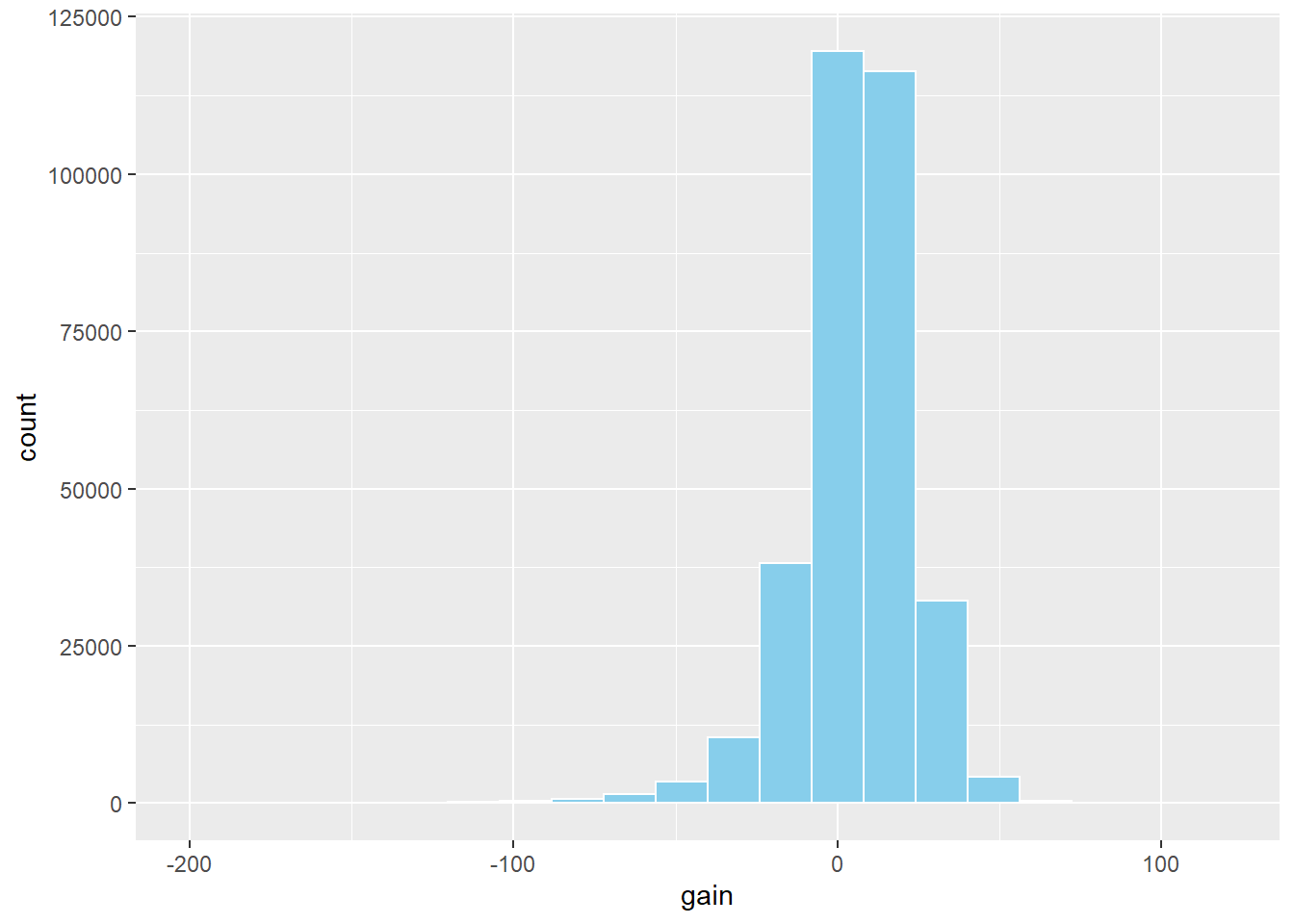

Figure 3: Histogram of gain variable

We can also create multiple columns at once and even refer to columns that were just created in a new column.

flights <- flights %>% 
  mutate(
    gain = dep_delay - arr_delay,
    hours = air_time / 60,
    gain_per_hour = gain / hours
  )
flights %>% 
  select(gain, hours, gain_per_hour) %>% 
  slice(1:5)

# A tibble: 5 x 3
   gain hours gain_per_hour
  <dbl> <dbl>         <dbl>
1    -9  3.78         -2.38
2   -16  3.78         -4.23
3   -31  2.67        -11.6 
4    17  3.05          5.57
5    19  1.93          9.83

Task What do positive values of the gain variable in flights correspond to? What about negative values? And what about a zero value?

Say a flight departed 20 minutes late, i.e. dep_delay = 20 then arrived 10 minutes late, i.e. arr_delay = 10. + Then gain = dep_delay - arr_delay = 20 - 10 = 10 is positive, so it "made up/gained time in the air". + 0 means the departure and arrival delays were the same, so no time was made up in the air.

We see in most cases that the gain is near 0 minutes.

Task Could we create the dep_delay and arr_delay columns by simply subtracting dep_time from sched_dep_time and similarly for arrivals? Try the code out and explain any differences between the result and what actually appears in flights.

No because you can't do direct arithmetic on times. The difference in time between 12:03 and 11:59 is 4 minutes, but 1203-1159 = 44

Task What can we say about the distribution of gain? Describe it in a few sentences using the plot and the gain_summary data frame values.

Most of the time the gain is between -25 and 25 minutes.
There are some extreme cases however, e.g. min(flights$gain, na.rm=T) returns -196 and max(flights$gain, na.rm=T) returns 109.

Create new variables/change old variables using mutate

Create new variables/change old variables using `mutate`