Joining data frames
Another common task is joining or merging two different data sets. For example, in the flights data, the variable carrier lists the carrier code for the different flights. While "UA" and "AA" might be somewhat easy to guess for some (United and American Airlines), what are "VX", "HA", and "B6"? This information is provided in a separate data frame airlines.
# A tibble: 6 × 2
  carrier name
  <chr>   <chr>
1 9E      Endeavor Air Inc.
2 AA      American Airlines Inc.
3 AS      Alaska Airlines Inc.
4 B6      JetBlue Airways
5 DL      Delta Air Lines Inc.
6 EV      ExpressJet Airlines Inc.
We see that in airports, carrier is the carrier code while name is the full name of the airline. Using this table, we can see that "VX", "HA", and "B6" correspond to Virgin America, Hawaiian Airlines, and JetBlue respectively. However, will we have to continually look up the carrier's name for each flight in the airlines data set? No! Instead of having to do this manually, we can have R automatically do the "looking up" for us.
Note that the values in the variable carrier in flights match the values in the variable carrier in airlines. In this case, we can use the variable carrier as a key variable to join/merge/match the two data frames by. Key variables are almost always identification variables that uniquely identify the observational units as we saw back in the "Identification vs Measurement Variable" section. This ensures that rows in both data frames are appropriate matched during the join.
This diagram helps us understand how the different data sets are linked by various key variables:
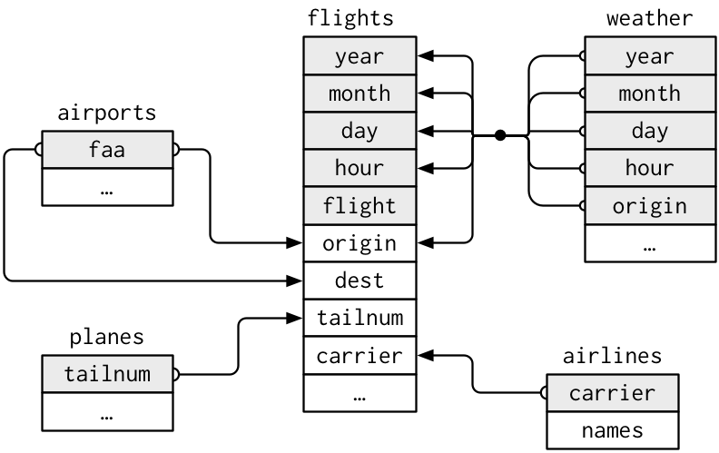
Figure 4: Data relationships in nycflights13 from R for Data Science, Hadley and Garrett (2016)
Joining by "key" variables
In both flights and airlines, the key variable we want to join/merge/match the two data frames with has the same name in both data sets: carriers. We make use of the inner_join() function to join by the variable carrier.
 [1] "year"           "month"          "day"            "dep_time"
 [5] "sched_dep_time" "dep_delay"      "arr_time"       "sched_arr_time"
 [9] "arr_delay"      "carrier"        "flight"         "tailnum"
[13] "origin"         "dest"           "air_time"       "distance"
[17] "hour"           "minute"         "time_hour"      "gain"
[21] "hours" "gain_per_hour" [1] "year" "month" "day" "dep_time"
[5] "sched_dep_time" "dep_delay" "arr_time" "sched_arr_time"
[9] "arr_delay" "carrier" "flight" "tailnum"
[13] "origin" "dest" "air_time" "distance"
[17] "hour" "minute" "time_hour" "gain"
[21] "hours" "gain_per_hour" "name" # A tibble: 336,776 × 3
flight carrier name
<int> <chr> <chr>
1 1545 UA United Air Lines Inc.
2 1714 UA United Air Lines Inc.
3 1141 AA American Airlines Inc.
4 725 B6 JetBlue Airways
5 461 DL Delta Air Lines Inc.
6 1696 UA United Air Lines Inc.
7 507 B6 JetBlue Airways
8 5708 EV ExpressJet Airlines Inc.
9 79 B6 JetBlue Airways
10 301 AA American Airlines Inc.
# ℹ 336,766 more rowsWe observed that the flights and flights_joined are identical except that flights_joined has an additional variable name whose values were drawn from airlines.
A visual representation of the inner_join is given below:
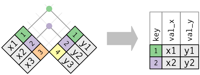
Figure 5: Diagram of inner join from R for Data Science
There are more complex joins available, but the inner_join will solve nearly all of the problems you'll face in our experience.
Joining by "key" variables with different names
Say instead, you are interested in all the destinations of flights from NYC in 2013 and ask yourself:
- "What cities are these airports in?"
- "Is
"ORD"Orlando?" - "Where is
"FLL"?
The airports data frame contains airport codes:
# A tibble: 6 × 8
  faa   name                             lat   lon   alt    tz dst   tzone
  <chr> <chr>                          <dbl> <dbl> <dbl> <dbl> <chr> <chr>
1 04G   Lansdowne Airport               41.1 -80.6  1044    -5 A     America/Ne…
2 06A   Moton Field Municipal Airport   32.5 -85.7   264    -6 A     America/Ch…
3 06C   Schaumburg Regional             42.0 -88.1   801    -6 A     America/Ch…
4 06N   Randall Airport                 41.4 -74.4   523    -5 A     America/Ne…
5 09J   Jekyll Island Airport           31.1 -81.4    11    -5 A     America/Ne…
6 0A9   Elizabethton Municipal Airport  36.4 -82.2  1593    -5 A     America/Ne…
However, looking at both the airports and flights and the visual representation of the relations between the data frames in the figure above, we see that in:
airportsthe airport code is in the variablefaaflightsthe departure airport code is in the variableorigin
So to join these two data sets, our inner_join operation involves a by argument that accounts for the different names:
Let's construct the sequence of commands that computes the number of flights from NYC to each destination, but also includes information about each destination airport:
named_dests <- flights %>%
  group_by(dest) %>%
  summarize(num_flights = n()) %>%
  arrange(desc(num_flights)) %>%
  inner_join(airports, by = c("dest" = "faa")) %>%
  rename(airport_name = name)
named_dests
# A tibble: 101 × 9
dest num_flights airport_name lat lon alt tz dst tzone
<chr> <int> <chr> <dbl> <dbl> <dbl> <dbl> <chr> <chr>
1 ORD 17283 Chicago Ohare Intl 42.0 -87.9 668 -6 A Amer…
2 ATL 17215 Hartsfield Jackson At… 33.6 -84.4 1026 -5 A Amer…
3 LAX 16174 Los Angeles Intl 33.9 -118. 126 -8 A Amer…
4 BOS 15508 General Edward Lawren… 42.4 -71.0 19 -5 A Amer…
5 MCO 14082 Orlando Intl 28.4 -81.3 96 -5 A Amer…
6 CLT 14064 Charlotte Douglas Intl 35.2 -80.9 748 -5 A Amer…
7 SFO 13331 San Francisco Intl 37.6 -122. 13 -8 A Amer…
8 FLL 12055 Fort Lauderdale Holly… 26.1 -80.2 9 -5 A Amer…
9 MIA 11728 Miami Intl 25.8 -80.3 8 -5 A Amer…
10 DCA 9705 Ronald Reagan Washing… 38.9 -77.0 15 -5 A Amer…
# ℹ 91 more rowsIn case you didn't know, "ORD" is the airport code of Chicago O'Hare airport and "FLL" is the main airport in Fort Lauderdale, Florida, which we can now see in our named_dests data frame.
Joining by multiple "key" variables
Say instead we are in a situation where we need to join by multiple variables. For example, in the first figure in this section we see that in order to join the flights and weather data frames, we need more than one key variable: year, month, day, hour, and origin. This is because the combination of these 5 variables act to uniquely identify each observational unit in the weather data frame: hourly weather recordings at each of the 3 NYC airports.
We achieve this by specifying a vector of key variables to join by using the c() concatenate function. Note the individual variables need to be wrapped in quotation marks.
flights_weather_joined <- flights %>%
  inner_join(weather, by = c("year", "month", "day", "hour", "origin"))
head(flights_weather_joined[,c(1:4,10:11,22:32)])
# A tibble: 6 × 17
year month day dep_time carrier flight gain_per_hour temp dewp humid
<int> <int> <int> <int> <chr> <int> <dbl> <dbl> <dbl> <dbl>
1 2013 1 1 517 UA 1545 -2.38 39.0 28.0 64.4
2 2013 1 1 533 UA 1714 -4.23 39.9 25.0 54.8
3 2013 1 1 542 AA 1141 -11.6 39.0 27.0 61.6
4 2013 1 1 544 B6 725 5.57 39.0 27.0 61.6
5 2013 1 1 554 DL 461 9.83 39.9 25.0 54.8
6 2013 1 1 554 UA 1696 -6.4 39.0 28.0 64.4
# ℹ 7 more variables: wind_dir <dbl>, wind_speed <dbl>, wind_gust <dbl>,
# precip <dbl>, pressure <dbl>, visib <dbl>, time_hour.y <dttm>Task
Looking at the first figure in this section, when joining flights and weather (or, in other words, matching the hourly weather values with each flight), why do we need to join by all of year, month, day, hour, and origin, and not just hour?
Because hour is simply a value between 0 and 23; to identify a specific hour, we need to also know which year, month, day and at which airport.