Other verbs
Select variables using select
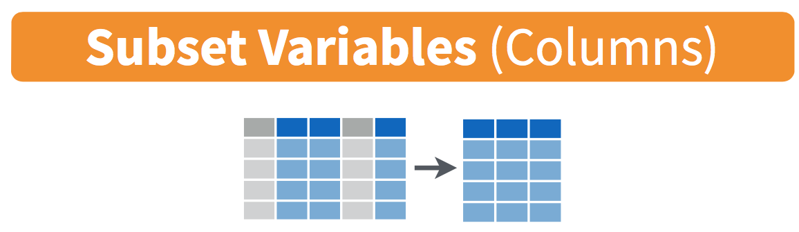
Figure 6: Select diagram from Data Wrangling with dplyr and tidyr cheatsheet
We've seen that the flights data frame in the nycflights13 package contains many different variables. The names function gives a listing of all the columns in a data frame; in our case you would run names(flights). You can also identify these variables by running the glimpse function in the dplyr package:
Rows: 336,776
Columns: 22
$ year           <int> 2013, 2013, 2013, 2013, 2013, 2013, 2013, 2013, 2013, 2…
$ month          <int> 1, 1, 1, 1, 1, 1, 1, 1, 1, 1, 1, 1, 1, 1, 1, 1, 1, 1, 1…
$ day            <int> 1, 1, 1, 1, 1, 1, 1, 1, 1, 1, 1, 1, 1, 1, 1, 1, 1, 1, 1…
$ dep_time       <int> 517, 533, 542, 544, 554, 554, 555, 557, 557, 558, 558, …
$ sched_dep_time <int> 515, 529, 540, 545, 600, 558, 600, 600, 600, 600, 600, …
$ dep_delay      <dbl> 2, 4, 2, -1, -6, -4, -5, -3, -3, -2, -2, -2, -2, -2, -1…
$ arr_time       <int> 830, 850, 923, 1004, 812, 740, 913, 709, 838, 753, 849,…
$ sched_arr_time <int> 819, 830, 850, 1022, 837, 728, 854, 723, 846, 745, 851,…
$ arr_delay      <dbl> 11, 20, 33, -18, -25, 12, 19, -14, -8, 8, -2, -3, 7, -1…
$ carrier        <chr> "UA", "UA", "AA", "B6", "DL", "UA", "B6", "EV", "B6", "…
$ flight         <int> 1545, 1714, 1141, 725, 461, 1696, 507, 5708, 79, 301, 4…
$ tailnum        <chr> "N14228", "N24211", "N619AA", "N804JB", "N668DN", "N394…
$ origin         <chr> "EWR", "LGA", "JFK", "JFK", "LGA", "EWR", "EWR", "LGA",…
$ dest           <chr> "IAH", "IAH", "MIA", "BQN", "ATL", "ORD", "FLL", "IAD",…
$ air_time       <dbl> 227, 227, 160, 183, 116, 150, 158, 53, 140, 138, 149, 1…
$ distance       <dbl> 1400, 1416, 1089, 1576, 762, 719, 1065, 229, 944, 733, …
$ hour           <dbl> 5, 5, 5, 5, 6, 5, 6, 6, 6, 6, 6, 6, 6, 6, 6, 5, 6, 6, 6…
$ minute         <dbl> 15, 29, 40, 45, 0, 58, 0, 0, 0, 0, 0, 0, 0, 0, 0, 59, 0…
$ time_hour      <dttm> 2013-01-01 05:00:00, 2013-01-01 05:00:00, 2013-01-01 0…
$ gain           <dbl> -9, -16, -31, 17, 19, -16, -24, 11, 5, -10, 0, 1, -9, 1…
$ hours          <dbl> 3.7833333, 3.7833333, 2.6666667, 3.0500000, 1.9333333, …
$ gain_per_hour  <dbl> -2.3788546, -4.2290749, -11.6250000, 5.5737705, 9.82758…
However, say you only want to consider two of these variables, say carrier and flight. You can select these:
# A tibble: 336,776 × 2
   carrier flight
   <chr>    <int>
 1 UA        1545
 2 UA        1714
 3 AA        1141
 4 B6         725
 5 DL         461
 6 UA        1696
 7 B6         507
 8 EV        5708
 9 B6          79
10 AA         301
# ℹ 336,766 more rows
This function makes navigating data sets with a very large number of variables easier for humans by restricting consideration to only those of interest, like carrier and flight above. So for example, this might make viewing the data set using the View() spreadsheet viewer more digestible. However, as far as the computer is concerned it doesn't care how many variables additional variables are in the data set in question, so long as carrier and flight are included.
Another example involves the variable year. If you remember the original description of the flights data frame (or by running ?flights), you'll remember that this data correspond to flights in 2013 departing New York City. The year variable isn't really a variable here in that it doesn't vary... flights actually comes from a larger data set that covers many years. We may want to remove the year variable from our data set since it won't be helpful for analysis in this case. We can deselect year by using the - sign:
 [1] "month"          "day"            "dep_time"       "sched_dep_time"
 [5] "dep_delay"      "arr_time"       "sched_arr_time" "arr_delay"
 [9] "carrier"        "flight"         "tailnum"        "origin"
[13] "dest"           "air_time"       "distance"       "hour"
[17] "minute"         "time_hour"      "gain"           "hours"
[21] "gain_per_hour"
Or we could specify a ranges of columns:
# A tibble: 336,776 × 5
   month   day dep_time arr_time sched_arr_time
   <int> <int>    <int>    <int>          <int>
 1     1     1      517      830            819
 2     1     1      533      850            830
 3     1     1      542      923            850
 4     1     1      544     1004           1022
 5     1     1      554      812            837
 6     1     1      554      740            728
 7     1     1      555      913            854
 8     1     1      557      709            723
 9     1     1      557      838            846
10     1     1      558      753            745
# ℹ 336,766 more rows
The select function can also be used to reorder columns in combination with the everything helper function. Let's suppose we'd like the hour, minute, and time_hour variables, which appear at the end of the flights data set, to actually appear immediately after the day variable:
flights_reorder <- flights %>%
  select(month:day, hour:time_hour, everything())
names(flights_reorder)
[1] "month" "day" "hour" "minute"
[5] "time_hour" "year" "dep_time" "sched_dep_time"
[9] "dep_delay" "arr_time" "sched_arr_time" "arr_delay"
[13] "carrier" "flight" "tailnum" "origin"
[17] "dest" "air_time" "distance" "gain"
[21] "hours" "gain_per_hour" in this case everything() picks up all remaining variables. Lastly, the helper functions starts_with, ends_with, and contains can be used to choose variables/column names that match those conditions:
# A tibble: 6 × 3
  arr_time arr_delay air_time
     <int>     <dbl>    <dbl>
1      830        11      227
2      850        20      227
3      923        33      160
4     1004       -18      183
5      812       -25      116
6 740 12 150# A tibble: 6 × 2
dep_delay arr_delay
<dbl> <dbl>
1 2 11
2 4 20
3 2 33
4 -1 -18
5 -6 -25
6 -4 12# A tibble: 6 × 6
dep_time sched_dep_time arr_time sched_arr_time air_time time_hour
<int> <int> <int> <int> <dbl> <dttm>
1 517 515 830 819 227 2013-01-01 05:00:00
2 533 529 850 830 227 2013-01-01 05:00:00
3 542 540 923 850 160 2013-01-01 05:00:00
4 544 545 1004 1022 183 2013-01-01 05:00:00
5 554 600 812 837 116 2013-01-01 06:00:00
6 554 558 740 728 150 2013-01-01 05:00:00Rename variables using rename
Another useful function is rename, which as you may suspect renames one column to another name. Suppose we wanted dep_time and arr_time to be departure_time and arrival_time instead in the flights_time data frame:
flights_time <- flights %>%
  select(contains("time")) %>%
  rename(departure_time = dep_time,
         arrival_time = arr_time)
names(flights_time)
[1] "departure_time" "sched_dep_time" "arrival_time" "sched_arr_time"
[5] "air_time" "time_hour" Note that in this case we used a single = sign with the rename(). e.g.. departure_time = dep_time. This is because we are not testing for equality like we would using ==, but instead we want to assign a new variable departure_time to have the same values as dep_time and then delete the variable dep_time.
It's easy to forget if the new name comes before or after the equals sign. I usually remember this as "New Before, Old After" or NBOA. You'll receive an error if you try to do it the other way:
Error: Unknown variables: departure_time, arrival_time.Find the top number of values using top_n
We can also use the top_n function which automatically tells us the most frequent num_flights. We specify the top 10 airports here:
# A tibble: 10 × 9
   dest  num_flights airport_name             lat    lon   alt    tz dst   tzone
   <chr>       <int> <chr>                  <dbl>  <dbl> <dbl> <dbl> <chr> <chr>
 1 MIA         11728 Miami Intl              25.8  -80.3     8    -5 A     Amer…
 2 FLL         12055 Fort Lauderdale Holly…  26.1  -80.2     9    -5 A     Amer…
 3 MCO         14082 Orlando Intl            28.4  -81.3    96    -5 A     Amer…
 4 ATL         17215 Hartsfield Jackson At…  33.6  -84.4  1026    -5 A     Amer…
 5 LAX         16174 Los Angeles Intl        33.9 -118.    126    -8 A     Amer…
 6 CLT         14064 Charlotte Douglas Intl  35.2  -80.9   748    -5 A     Amer…
 7 SFO         13331 San Francisco Intl      37.6 -122.     13    -8 A     Amer…
 8 DCA          9705 Ronald Reagan Washing…  38.9  -77.0    15    -5 A     Amer…
 9 ORD         17283 Chicago Ohare Intl      42.0  -87.9   668    -6 A     Amer…
10 BOS         15508 General Edward Lawren…  42.4  -71.0    19    -5 A     Amer…
We'll still need to arrange this by num_flights though:
# A tibble: 10 × 9
   dest  num_flights airport_name             lat    lon   alt    tz dst   tzone
   <chr>       <int> <chr>                  <dbl>  <dbl> <dbl> <dbl> <chr> <chr>
 1 ORD         17283 Chicago Ohare Intl      42.0  -87.9   668    -6 A     Amer…
 2 ATL         17215 Hartsfield Jackson At…  33.6  -84.4  1026    -5 A     Amer…
 3 LAX         16174 Los Angeles Intl        33.9 -118.    126    -8 A     Amer…
 4 BOS         15508 General Edward Lawren…  42.4  -71.0    19    -5 A     Amer…
 5 MCO         14082 Orlando Intl            28.4  -81.3    96    -5 A     Amer…
 6 CLT         14064 Charlotte Douglas Intl  35.2  -80.9   748    -5 A     Amer…
 7 SFO         13331 San Francisco Intl      37.6 -122.     13    -8 A     Amer…
 8 FLL         12055 Fort Lauderdale Holly…  26.1  -80.2     9    -5 A     Amer…
 9 MIA         11728 Miami Intl              25.8  -80.3     8    -5 A     Amer…
10 DCA          9705 Ronald Reagan Washing…  38.9  -77.0    15    -5 A     Amer…
Note: Remember that I didn't pull the n and wt arguments out of thin air. They can be found by using the ? function on top_n.
We can go one step further and tie together the group_by and summarize functions we used to find the most frequent flights:
ten_freq_dests <- flights %>%
  group_by(dest) %>%
  summarize(num_flights = n()) %>%
  arrange(desc(num_flights)) %>%
  top_n(n = 10)
ten_freq_dests
# A tibble: 10 × 2
dest num_flights
<chr> <int>
1 ORD 17283
2 ATL 17215
3 LAX 16174
4 BOS 15508
5 MCO 14082
6 CLT 14064
7 SFO 13331
8 FLL 12055
9 MIA 11728
10 DCA 9705Task
What are some ways to select all three of the dest, air_time, and distance variables from flights? Give the code showing how to do this in at least three different ways.
# A tibble: 336,776 × 3
   dest  air_time distance
   <chr>    <dbl>    <dbl>
 1 IAH        227     1400
 2 IAH        227     1416
 3 MIA        160     1089
 4 BQN        183     1576
 5 ATL        116      762
 6 ORD        150      719
 7 FLL        158     1065
 8 IAD         53      229
 9 MCO        140      944
10 ORD        138      733
# ℹ 336,766 more rows# A tibble: 336,776 × 3
dest air_time distance
<chr> <dbl> <dbl>
1 IAH 227 1400
2 IAH 227 1416
3 MIA 160 1089
4 BQN 183 1576
5 ATL 116 762
6 ORD 150 719
7 FLL 158 1065
8 IAD 53 229
9 MCO 140 944
10 ORD 138 733
# ℹ 336,766 more rowsflights %>%
select(-year, -month, -day, -dep_time, -sched_dep_time, -dep_delay, -arr_time,
-sched_arr_time, -arr_delay, -carrier, -flight, -tailnum, -origin,
-hour, -minute, -time_hour)# A tibble: 336,776 × 6
dest air_time distance gain hours gain_per_hour
<chr> <dbl> <dbl> <dbl> <dbl> <dbl>
1 IAH 227 1400 -9 3.78 -2.38
2 IAH 227 1416 -16 3.78 -4.23
3 MIA 160 1089 -31 2.67 -11.6
4 BQN 183 1576 17 3.05 5.57
5 ATL 116 762 19 1.93 9.83
6 ORD 150 719 -16 2.5 -6.4
7 FLL 158 1065 -24 2.63 -9.11
8 IAD 53 229 11 0.883 12.5
9 MCO 140 944 5 2.33 2.14
10 ORD 138 733 -10 2.3 -4.35
# ℹ 336,766 more rowsTask
How could one use starts_with, ends_with, and contains to select columns from the flights data frame? Provide three different examples in total: one for starts_with, one for ends_with, and one for contains.
# A tibble: 336,776 × 5
     day dep_time dep_delay dest  distance
   <int>    <int>     <dbl> <chr>    <dbl>
 1     1      517         2 IAH       1400
 2     1      533         4 IAH       1416
 3     1      542         2 MIA       1089
 4     1      544        -1 BQN       1576
 5     1      554        -6 ATL        762
 6     1      554        -4 ORD        719
 7     1      555        -5 FLL       1065
 8     1      557        -3 IAD        229
 9     1      557        -3 MCO        944
10     1      558        -2 ORD        733
# ℹ 336,766 more rows
# A tibble: 336,776 × 2
dep_delay arr_delay
<dbl> <dbl>
1 2 11
2 4 20
3 2 33
4 -1 -18
5 -6 -25
6 -4 12
7 -5 19
8 -3 -14
9 -3 -8
10 -2 8
# ℹ 336,766 more rows# A tibble: 336,776 × 3
dep_time sched_dep_time dep_delay
<int> <int> <dbl>
1 517 515 2
2 533 529 4
3 542 540 2
4 544 545 -1
5 554 600 -6
6 554 558 -4
7 555 600 -5
8 557 600 -3
9 557 600 -3
10 558 600 -2
# ℹ 336,766 more rowsTask Create a new data frame that shows the top 5 airports with the largest average arrival delays from NYC in 2013.
top5_arr_delays <- flights %>%
  group_by(dest) %>%
  summarize(mean_arr_delay = mean(arr_delay, na.rm=T)) %>%
  arrange(desc(mean_arr_delay)) %>%
  top_n(n = 5)

top5_arr_delays %>%
  inner_join(airports %>% select(faa, name), by = c("dest" = "faa") )
# A tibble: 5 × 3
dest mean_arr_delay name
<chr> <dbl> <chr>
1 CAE 41.8 Columbia Metropolitan
2 TUL 33.7 Tulsa Intl
3 OKC 30.6 Will Rogers World
4 JAC 28.1 Jackson Hole Airport
5 TYS 24.1 Mc Ghee Tyson