Summary
The table below lists a selection of the data wrangling verbs and summarizes what they do. Using these verbs and the pipe %>% operator, you'll be able to write easily legible code to perform almost all the data wrangling necessary for the rest of this course.
| Verb | Operation |
|---|---|
| filter() | Pick out a subset of rows |
| summarize() | Summarize many values to one using a summary statistic function like mean(), median(), etc. |
| group_by() | Add grouping structure to rows in data frame. Note this does not change values in data frame. |
| mutate() | Create new variables by mutating existing ones |
| arrange() | Arrange rows of a data variable in ascending (default) or descending order |
| inner_join() | Join/merge two data frames, matching rows by a key variable |
| select() | Pick out a subset of columns to make data frames easier to view |
Task An airline industry measure of a passenger airline's capacity is the available seat miles, which is equal to the number of seats available multiplied by the number of miles or kilometers flown. So for example say an airline had 2 flights using a plane with 10 seats that flew 500 miles and 3 flights using a plane with 20 seats that flew 1000 miles, the available seat miles would be 2 \(\times\) 10 \(\times\) 500 \(+\) 3 \(\times\) 20 \(\times\) 1000 = 70,000 seat miles.
Using the data sets included in the nycflights13 package, compute the available seat miles for each airline sorted in descending order. After completing all the necessary data wrangling steps, the resulting data frame should have 16 rows (one for each airline) and 2 columns (airline name and available seat miles). Here are some hints:
Crucial: Unless you are very confident in what you are doing, it is worthwhile to not start coding right away. Rather first sketch out on paper all the necessary data wrangling steps, not using exact code, but rather high-level pseudocode that is informal yet detailed enough to articulate what you are doing. This way you won't confuse what you are trying to do (the algorithm) with how you are going to do it (writing
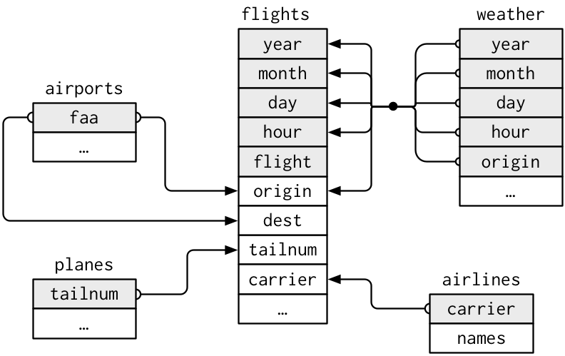
dplyrcode).Take a close look at all the data sets using the
View(),head()orglimpse()functions:flights,weather,planes,airports, andairlinesto identify which variables are necessary to compute available seat miles.This diagram (from the "Joining section"") will also be useful.
Consider the data wrangling verbs in the table above as your toolbox!
If you want to work through it step by step, here are some hints:
Step 1: To compute the available seat miles for a given flight, we need the distance variable from the flights data frame and the seats variable from the planes data frame, necessitating a join by the key variable tailnum. To keep the resulting data frame easy to view, we'll select() only these two variables and carrier.
# A tibble: 284,170 × 3
carrier seats distance
<chr> <int> <dbl>
1 UA 149 1400
2 UA 149 1416
3 AA 178 1089
4 B6 200 1576
5 DL 178 762
6 UA 191 719
7 B6 200 1065
8 EV 55 229
9 B6 200 944
10 B6 200 1028
# ℹ 284,160 more rowsStep 2: Now for each flight we can compute the available seat miles ASM by multiplying the number of seats by the distance via a mutate().
flights %>%
  inner_join(planes, by = "tailnum") %>%
select(carrier, seats, distance) %>%
mutate(ASM = seats * distance)# A tibble: 284,170 × 4
carrier seats distance ASM
<chr> <int> <dbl> <dbl>
1 UA 149 1400 208600
2 UA 149 1416 210984
3 AA 178 1089 193842
4 B6 200 1576 315200
5 DL 178 762 135636
6 UA 191 719 137329
7 B6 200 1065 213000
8 EV 55 229 12595
9 B6 200 944 188800
10 B6 200 1028 205600
# ℹ 284,160 more rowsStep 3: Next we want to sum the ASM for each carrier. We achieve this by first grouping by carrier and then summarizing using the sum() function.
flights %>%
  inner_join(planes, by = "tailnum") %>%
  select(carrier, seats, distance) %>%
mutate(ASM = seats * distance) %>%
# Added:
group_by(carrier) %>%
summarize(ASM = sum(ASM))# A tibble: 16 × 2
carrier ASM
<chr> <dbl>
1 9E 776970310
2 AA 3677292231
3 AS 314104736
4 B6 9618222135
5 DL 10532885801
6 EV 1817236275
7 F9 184832280
8 FL 219628520
9 HA 642478122
10 MQ 7162420
11 OO 1299835
12 UA 15516377526
13 US 2533505829
14 VX 2296680778
15 WN 1718116857
16 YV 20163632Step 4: However, if it was the case that some carriers had certain flights with missing NA values, the resulting table above would also returns NA's (NB: this is not the case for this data). We can eliminate these by adding a na.rm = TRUE argument to sum(), telling R that we want to remove the NA's in the sum.
flights %>%
  inner_join(planes, by = "tailnum") %>%
  select(carrier, seats, distance) %>%
  mutate(ASM = seats * distance) %>%
  group_by(carrier) %>%
  # Modified:
  summarize(ASM = sum(ASM, na.rm = TRUE))
# A tibble: 16 × 2
carrier ASM
<chr> <dbl>
1 9E 776970310
2 AA 3677292231
3 AS 314104736
4 B6 9618222135
5 DL 10532885801
6 EV 1817236275
7 F9 184832280
8 FL 219628520
9 HA 642478122
10 MQ 7162420
11 OO 1299835
12 UA 15516377526
13 US 2533505829
14 VX 2296680778
15 WN 1718116857
16 YV 20163632Step 5: Finally, we arrange() the data in desc()ending order of ASM.
flights %>%
  inner_join(planes, by = "tailnum") %>%
  select(carrier, seats, distance) %>%
  mutate(ASM = seats * distance) %>%
  group_by(carrier) %>%
  summarize(ASM = sum(ASM, na.rm = TRUE)) %>%
  arrange(desc(ASM))
# A tibble: 16 × 2
carrier ASM
<chr> <dbl>
1 UA 15516377526
2 DL 10532885801
3 B6 9618222135
4 AA 3677292231
5 US 2533505829
6 VX 2296680778
7 EV 1817236275
8 WN 1718116857
9 9E 776970310
10 HA 642478122
11 AS 314104736
12 FL 219628520
13 F9 184832280
14 YV 20163632
15 MQ 7162420
16 OO 1299835